(Archived Original Version) Spherical Gaussian Encoding
Note: this was the originally posted version of the running average algorithm. See the updated post for a more accurate version.
Spherical Gaussians are a useful tool for encoding precomputed radiance within a scene. Matt Pettineo has an excellent series describing the technical details and history behind them which I’d suggest reading before the rest of this post.
Recently, I’ve had need to build spherical Gaussian representations of a scene on the fly in the GPU path tracer I’m building for my Master’s project. Unlike, say, spherical harmonics, spherical Gaussian lobes don’t form a set of orthonormal bases; they need to be computed with a least-squares solve, which generally requires having access to all radiance samples at once (although, as Peter-Pike Sloan points out on Twitter, that doesn’t always have to be the case). On the GPU, in a memory-constrained environment, this is highly impractical.
Instead, games like The Order: 1886 just projected the samples onto the spherical Gaussian lobes as if the lobes form an orthonormal basis, which gave low-quality results that lack contrast. For my research, I wanted to see if I could do better.
After a bunch of experimentation, I found a new algorithm for accumulating spherical Gaussian samples that’s almost as good as a least-squares solve if the sample directions are randomly distributed, or is slightly better than a naïve projection if the sample directions are correlated (as they would be, say, if you were reading pixels row by row from a lat-long image map.) Conveniently, when we’re accumulating samples from path tracing the sample directions are usually stratified or uniformly random.
One note of caution: some low-discrepancy sequences (e.g. fixed-length ones like the Hammersley sequence) will not work well if successive samples are correlated, even though the sequence is well-distributed over the entire domain.
The algorithm is as follows, and supports both non-negative and regular solves:
struct SphericalGaussianBasis {
    var lobes : [SphericalGaussian]
    var lobeWeights = [Float](repeating: 0.0, count: lobes.count)
    let nonNegativeSolve : Bool

    mutating func accumulateSample(_ sample: RadianceSample) {
        var currentValue = float3(0)

        var sampleLobeWeights = [Float](repeating: 0.0, count: self.lobes.count)
        for (i, lobe) in self.lobes.enumerated() {
            let dotProduct = dot(lobe.axis, sample.direction)
            let weight = exp(lobe.sharpness * (dotProduct - 1.0))
            currentValue += lobe.amplitude * weight

            sampleLobeWeights[i] = weight
        }

        let deltaValue = sample.value - currentValue

        for i in 0..<self.lobes.count {
            let weight = sampleLobeWeights[i]
            if weight == 0 { continue }

            lobeWeights[i] += weight

            let weightScale = weight / self.lobeWeights[i]
            self.lobes[i].amplitude += deltaValue * weightScale

            if (self.nonNegativeSolve) {
                self.lobes[i].amplitude = max(self.lobes[i].amplitude, float3(0))
            }
        }
    }
}
The basic idea is fairly simple: at each step, we evaluate the sum of the spherical Gaussian lobes in the new sample’s direction. Then, we evaluate the difference between the sample’s value and the current value. Finally, we adjust each lobe’s amplitude towards the sample’s amplitude according to its weight. If we want the lobe to be non-negative, we simply clamp it; the next sample to come in will then be evaluated against the set of non-negative lobes. I’ve called this a ‘running average’; perhaps a better description is that is uses gradient descent to solve for the radiance.
So how does it look? Well, here are the results for the ‘ennis.hdr’ environment map using uniformly randomly shuffled sample directions and twelve lobes (‘Running Average’ is my new method):
| Radiance | Irradiance | Irradiance Error (sMAPE) | Encoding Method |
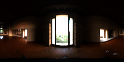 |  | Reference | |
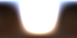
 RMS: 4.24835 | 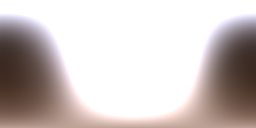 RMS: 0.441404 | 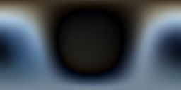 | Naïve |
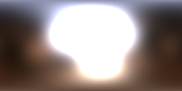
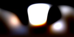 RMS: 3.80738 | 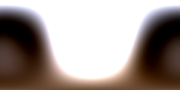 RMS: 0.228353 | 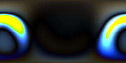 | Least Squares |
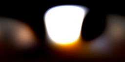 RMS: 3.81673 | 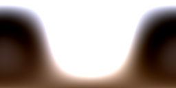 RMS: 0.221796 | 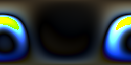 | Running Average |
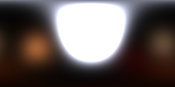 RMS: 3.9339 | 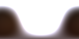 RMS: 0.786142 | 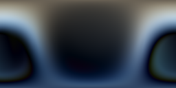 | Non-Negative Least Squares |
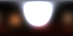 RMS: 3.92593 | 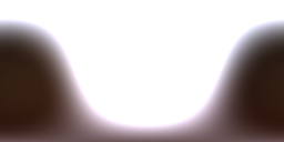 RMS: 0.670631 |  | Non-Negative Running Average |
It’s a marked improvement over the naïve projection, and, depending on the sample distribution, can be imperceptibly different from a standard least squares solve. And it all works on the fly, on the GPU, requiring only a per-lobe mean and weight to be stored.
In these images, I’m using Stephen Hill’s fitted approximation for a cosine lobe to evaluate the irradiance for all encoding methods.
Update: Matt Pettineo has integrated this new method into The Baking Lab. If you want to take a look you can find it under the ‘Running Average’ and ‘Running Average Non-Negative’ solve modes.
As I progress on my thesis, I hope to uncover more of the reasoning behind why it works so well, and I’m also hopeful it can find applications for this in other encoding schemes (Ambient Dice, perhaps?).
While testing this, I used Probulator, a useful open-source tool for testing different lighting encoding strategies. The source code for the implementation of this method within Probulator is below.
Note that the original implementation of irradiance for the naïve projection in Probulator cheats a little bit since it uses a non-cosine BRDF to evaluate the spherical Gaussian lobes. If we’re also using the spherical Gaussian to encode radiance for specular lighting, compensating with the BRDF doesn’t really work; we want things to be consistent.
class ExperimentSGRunningAverage : public ExperimentSGBase
{
public:
  void solveForRadiance(const std::vector<RadianceSample>& _radianceSamples) override
  {
      const u32 lobeCount = (u32)m_lobes.size();

      float lobeWeights[lobeCount];

      for (u32 lobeIt = 0; lobeIt < lobeCount; ++lobeIt) {
          lobeWeights[lobeIt] = 0.f;
      }

      std::vector<RadianceSample> radianceSamples = _radianceSamples;
      // The samples should be uniformly randomly distributed (or stratified) for best results.
      std::random_shuffle(radianceSamples.begin(), radianceSamples.end());

      for (size_t sampleIdx = 0; sampleIdx < radianceSamples.size(); sampleIdx += 1) {
          const RadianceSample& sample = radianceSamples[sampleIdx];

          vec3 currentValue = vec3(0.f);

          float sampleLobeWeights[lobeCount];
          for (u32 lobeIt = 0; lobeIt < lobeCount; ++lobeIt) {
              float dotProduct = dot(m_lobes[lobeIt].p, sample.direction);
              float weight = exp(m_lobes[lobeIt].lambda * (dotProduct - 1.0));
              currentValue += m_lobes[lobeIt].mu * weight;

              sampleLobeWeights[lobeIt] = weight;
          }

          vec3 deltaValue = sample.value - currentValue;

          for (u32 lobeIt = 0; lobeIt < lobeCount; ++lobeIt) {
              float weight = sampleLobeWeights[lobeIt];
              if (weight == 0.f) { continue; }

              lobeWeights[lobeIt] += weight;

              float weightScale = weight / lobeWeights[lobeIt];
              m_lobes[lobeIt].mu += deltaValue * weightScale;

              if (m_nonNegativeSolve) {
                  m_lobes[lobeIt].mu = max(m_lobes[lobeIt].mu, vec3(0.f));
              }
          }
      }
  }
}