Spherical Gaussian Encoding
Update: This post has now been published in paper form as “Progressive Least-Squares Encoding for Linear Bases” in the open-access journal JCGT. Take a look there for a more formalised derivation and more details.
Spherical Gaussians are a useful tool for encoding precomputed radiance within a scene. Matt Pettineo has an excellent series describing the technical details and history behind them which I’d suggest reading before the rest of this post.
Recently, I’ve had need to build spherical Gaussian representations of a scene on the fly in the GPU path tracer I’m building for my Master’s project. Unlike, say, spherical harmonics, spherical Gaussian lobes don’t form a set of orthonormal bases; they need to be computed with a least-squares solve, which is generally1 done with access to all radiance samples at once. On the GPU, in a memory-constrained environment, this is highly impractical.
Instead, games like The Order: 1886 just projected the samples onto the spherical Gaussian lobes as if the lobes form an orthonormal basis, which gave low-quality results that lack contrast. For my research, I wanted to see if I could do better.
After a bunch of experimentation, I found a new (to my knowledge) algorithm for progressively accumulating spherical Gaussian samples that gives results matching a standard least squares solve.
The algorithm is as follows, and supports both non-negative and regular solves. While the implementation focuses on spherical Gaussians, the algorithm should work for any set of spherical basis functions, provided those basis functions don’t overlap too much.
struct SphericalGaussianBasis {
    var lobes : [SphericalGaussian]
    var totalAccumulatedWeight : Float = 0.0
    var lobeMCSphericalIntegrals = [Float](repeating: 0.0, count: lobes.count) // Optional, can be precomputed at a slight increase in error.
    let nonNegativeSolve : Bool

    mutating func accumulateSample(_ sample: RadianceSample, sampleWeight: Float = 1.0) {
        totalAccumulatedWeight += sampleWeight
        let sampleWeightScale = sampleWeight / totalAccumulatedWeight

        var delta = sample.value

        var sampleLobeWeights = [Float](repeating: 0.0, count: self.lobes.count)
        for (i, lobe) in self.lobes.enumerated() {
            let dotProduct = dot(lobe.axis, sample.direction)
            let weight = exp(lobe.sharpness * (dotProduct - 1.0))
            delta -= lobe.amplitude * weight

            sampleLobeWeights[i] = weight
        }

        for i in 0..<self.lobes.count {
            let weight = sampleLobeWeights[i]

            let sphericalIntegralGuess = weight * weight

            // Update the MC-computed integral of the lobe over the domain.
            self.lobeMCSphericalIntegrals[i] += (sphericalIntegralGuess - self.lobeMCSphericalIntegrals[i]) * sampleWeightScale

            // The most accurate method requires using the MC-computed integral,
            // since then bias in the estimate will partially cancel out.
            // However, if you don't want to store a weight per-lobe you can instead substitute it with the
            // precomputed integral at a slight increase in error.

            // Interpolate from 1 to the true spherical integral as the sample count increases to avoid excess noise
            // in the early estimates.
            let sphericalIntegral = sampleWeightScale + (1 - sampleWeightScale) * self.lobeMCSphericalIntegrals[i]

            // Alternatively, you can also use this for the spherical integral:
            // let sphericalIntegral = max(self.lobeMCSphericalIntegrals[i], self.lobes[i].precomputedSphericalIntegral)

            // The acceleration coefficient helps to avoid local minima, although it can make the solve noisier.
            // 3.0 seems to be a good value in my tests; 1.0 means no acceleration.
            let accelerationCoefficient : Float = 3.0

            let deltaScale = accelerationCoefficient * sampleWeightScale * weight / sphericalIntegral
            self.lobes[i].amplitude += delta * deltaScale

            if (self.nonNegativeSolve) {
                self.lobes[i].amplitude = max(self.lobes[i].amplitude, float3(0))
            }

            // Optional, slightly improves convergence:
            // This step is more important when the lobes overlap significantly:
            delta *= 1.0 - deltaScale * weight
        }
    }
}
I’ve called this a ‘running average’ since each new sample is evaluated against the Monte-Carlo estimate of the function based on the previous samples. If we want each lobe to be non-negative, we simply clamp it; the next sample to come in will then be evaluated against the set of non-negative lobes.
I provide a mathematical derivation of the method here.
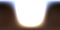
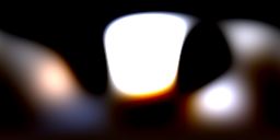
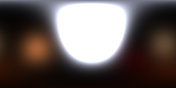
So how does it look? Well, here are the results for the ‘ennis.hdr’ environment map using Halton-sequence sample directions and twelve lobes, where ‘Running Average’ is my new method. In these images, I’m using Stephen Hill’s fitted approximation for a cosine lobe to evaluate the irradiance for all encoding methods.
| Radiance | Irradiance | Irradiance Error (sMAPE) | Encoding Method |
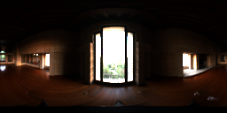 |  | Reference | |
 RMS: 4.24341 | 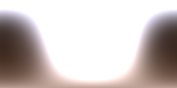 RMS: 0.44259 | 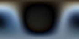 | Naïve |
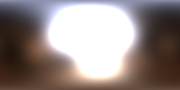
 RMS: 3.81043 | 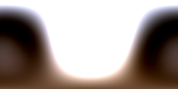 RMS: 0.241267 | 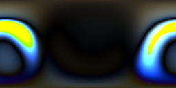 | Least Squares |
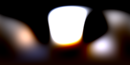 RMS: 3.80723 | 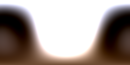 RMS: 0.243617 | 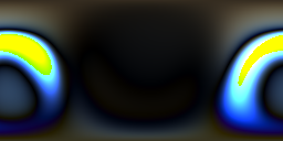 | Running Average |
 RMS: 3.93677 |  RMS: 0.808848 |  | Non-Negative Least Squares |
 RMS: 3.93653 |  RMS: 0.807047 |  | Non-Negative Running Average |
It’s a marked improvement over the naïve projection, and, depending on the sample distribution, can even achieve results as good as a standard least squares solve. And it all works on the fly, on the GPU, requiring only a per-lobe mean and the total sample weight for all lobes to be stored. For best quality, I recommend also storing a per-lobe estimate of the spherical integral, as is done above; however, that can be replaced with the precomputed spherical integral at a small increase in error.
The precomputed spherical integrals referenced in the code above are the integral of each basis function (e.g. each SG lobe) squared over the sampling domain. If the samples are distributed over a sphere then this has a closed-form solution; otherwise it can be precomputed using Monte-Carlo integration. Note that I’ve omitted dividing by the sampling PDF since the factors cancel out with the sampling in my algorithm above.
struct SphericalGaussian {
    var amplitude : float3
    var axis : float3
    var sharpness : Float

    var sphericalIntegral : Float {
        return (1.0 - exp(-4.0 * self.sharpness)) / (4.0 * self.sharpness)
    }

    var hemisphericalIntegral : Float {
        var total = 0.0 as Float
        let sampleCount = 2048

        for _ in 0..<sampleCount {
            let direction = float3.randomOnHemisphere

            let dotProduct = dot(self.axis, direction)
            let weight = exp(self.sharpness * (dotProduct - 1.0))
            total += weight * weight
        }

        return total / Float(sampleCount)
    }
}
I originally posted a variant of this algorithm that contained a few approximations. After that post, Peter-Pike Sloan pointed out on Twitter that least squares doesn’t necessarily require all samples to be stored; instead, you can accumulate the raw moments and then multiply by a lobeCount × lobeCount matrix to reconstruct the result. I realised my method was effectively an online approximation to this, and was able to correct a couple of approximations to bring it to match the equation.
The results are now as good as a standard least-squares solve if the sample directions are randomly distributed, although it does deteriorate if the sample directions are correlated (as they would be, say, if you were reading pixels row by row from a lat-long image map). Conveniently, when we’re accumulating samples from path tracing the sample directions are usually stratified or uniformly random. 2
This method does require at least 32-bit intermediates for accumulation; half-precision produces obvious visual artefacts and biasing towards high-intensity samples.
While testing this, I used Probulator, a useful open-source tool for testing different lighting encoding strategies. This method has also been merged into Probulator, and the source can be viewed here.
If you want to see this method running in a lightmap baking context, Matt Pettineo has integrated it into The Baking Lab. You can find it under the ‘Running Average’ and ‘Running Average Non-Negative’ solve modes.
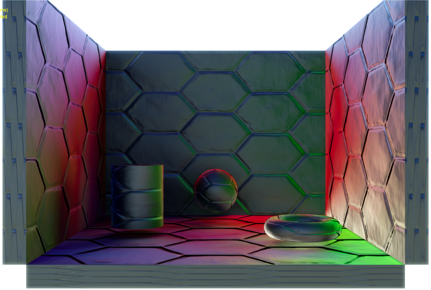
Below is a comparison from within The Baking Lab of the indirect specular from nine spherical Gaussian lobes using 10,000 samples per texel. The exposure has been turned up to more clearly show the results. There are slight visual differences if you flick back and forward, but it’s very close! The main difference is that the running average algorithm can find different local minima per-texel, and so results appear noisier across the texels.
Running Average:

Least Squares:
The code above has been factorised to try to limit the number of operations on colours. For example, the lines:
let deltaScale = accelerationCoefficient * sampleWeightScale * weight / sphericalIntegral
self.lobes[i] += delta * deltaScale
are more naturally expressed as:
let projection = self.lobes[i].amplitude * weight
let newValue = (delta + projection) * weight / sphericalIntegral
self.lobes[i].amplitude += (newValue - self.lobes[i].amplitude) * sampleWeightScale
These two snippets aren’t exactly equivalent. In factorising the code, I approximated highlight swiftprojection * weight * weight / sphericalIntegral as simply projection; it turns out that making this approximation helps to avoid error in the method. To make them equivalent, the first snippet would be:
let dampingTerm = 1.0 + (deltaScale * weight - sampleWeightScale)
self.lobes[i].amplitude *= dampingTerm

let deltaScale = accelerationCoefficient * sampleWeightScale * weight / sphericalIntegral
self.lobes[i] += delta * deltaScale
Similarly,
delta *= 1.0 - deltaScale * weightis equivalent to:
let oldAmplitude = self.lobes[i].amplitude - delta * deltaScale
delta = delta + oldAmplitude * weight - self.lobes[i].amplitude * weight-
It’s possible to perform least squares on the raw moments (the naïve projection) by multiplying by the inverse of the Gram matrix, as is alluded to later in this post. ↩
-
One note of caution: some low-discrepancy sequences (e.g. fixed-length ones like the Hammersley sequence) will not work well since successive samples are correlated, even though the sequence is well-distributed over the entire domain. One way around this is to uniformly randomly shuffle the samples. ↩