Spherical Radial Basis Functions for Lighting
| Indirect lighting from baked lightmaps in Crytek Sponza with only single-scattering GGX specular materials |
|---|
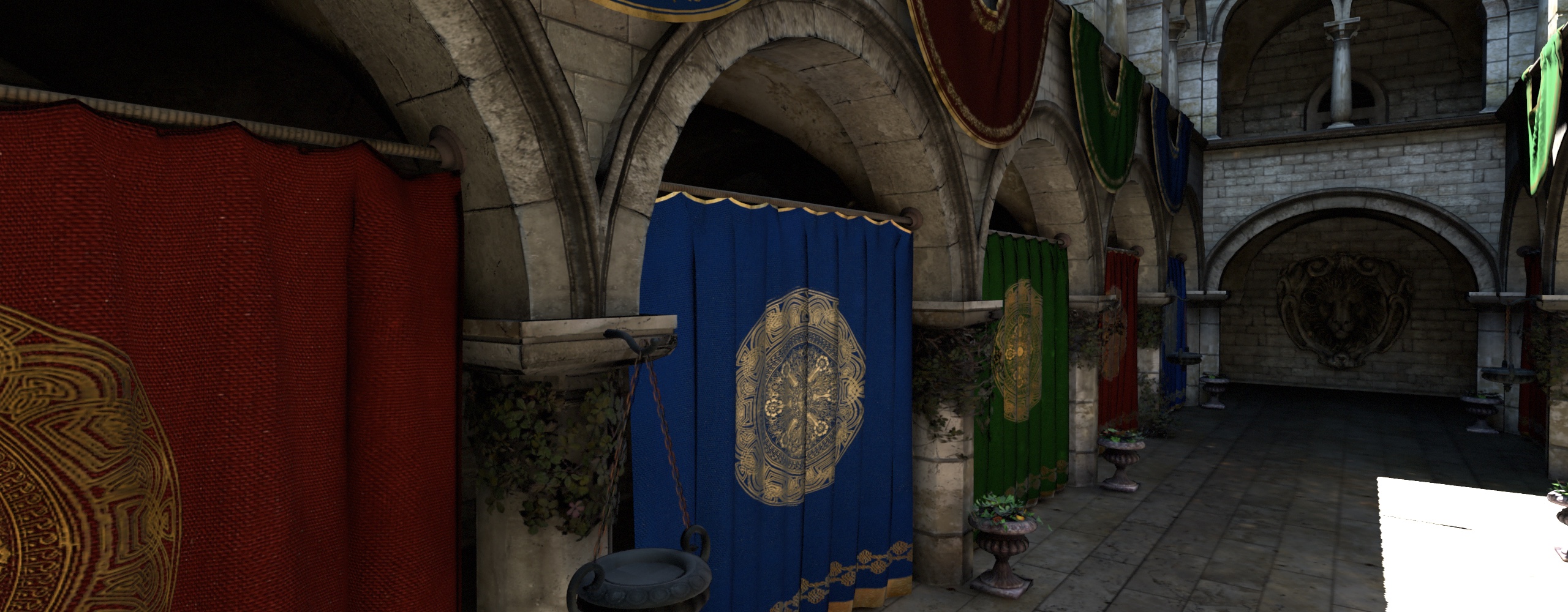 |
| Non-negative hemispherical Ambient Dice (nine lobes) (0.9ms per frame) |
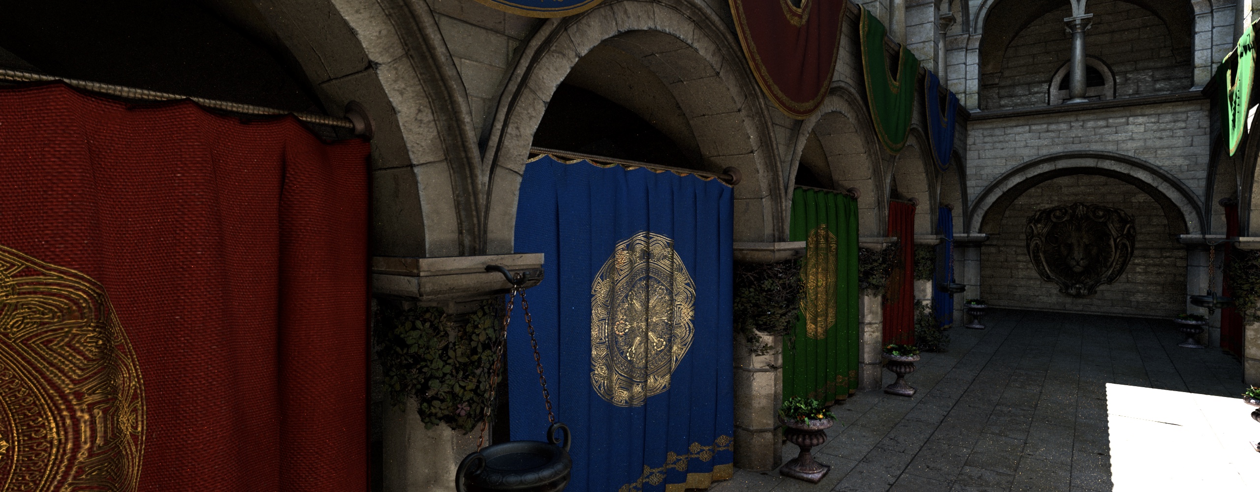 |
| Path-traced reference |
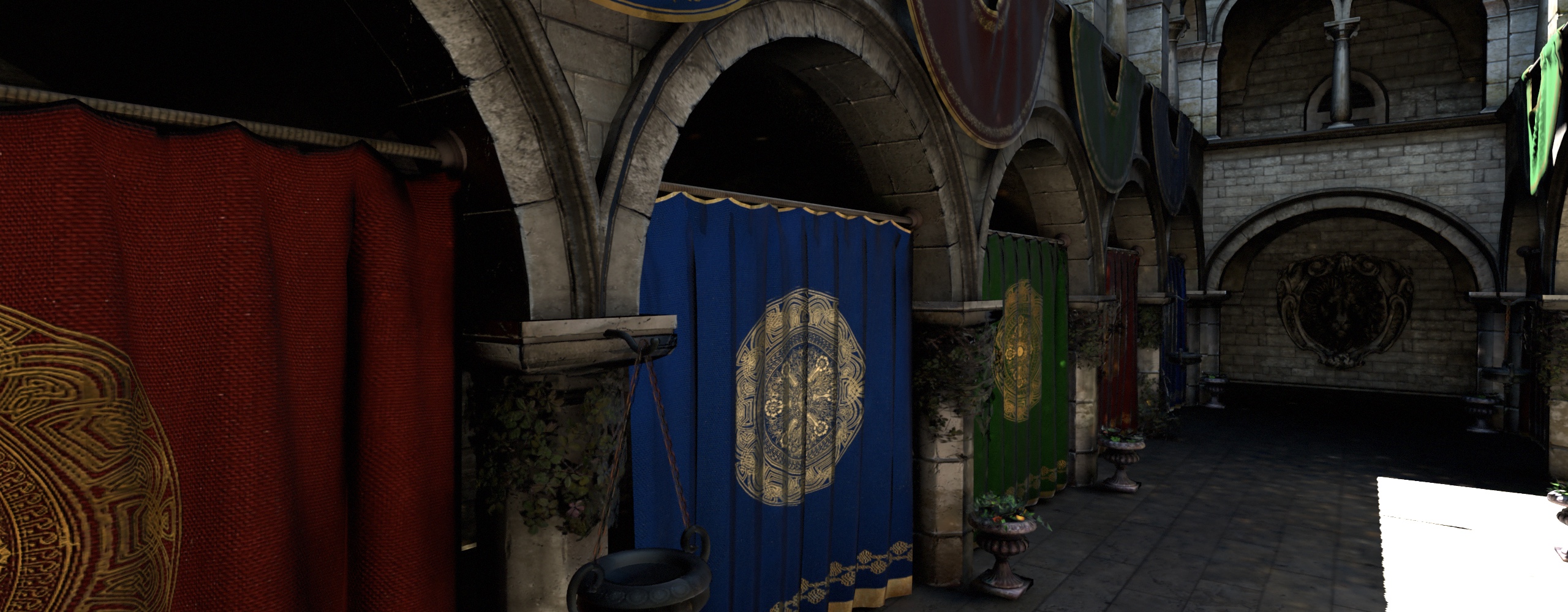 |
| Non-negative spherical Gaussians (twelve lobes, \(\lambda = 8\)) (2.5ms per frame) |
With my thesis now published, I wanted to break down one of its key contributions: namely, the extension of Iwanicki and Sloan’s Ambient Dice basis function to store and evaluate both diffuse and specular irradiance. This content mainly comes from Chapters 7 & 8 of the thesis.
Firstly, it’s worth quickly covering what linear bases are. When we add multiple functions \(B_i(s)\) together and multiply by basis coefficients \(b_i\), we get a linear basis, where \(B_i(s)\) is the \(i^{th}\) basis function of the linear basis:
\[\sum_i b_i B_i(s)\]Determining the basis coefficient vector \(b\) that best fits some function \(f(s)\) such that
\[f(s) \approx \sum_i b_i B_i(s)\]can be done by least-squares encoding; essentially, least-squares encoding tries to find the coefficients \(b\) that will enable the weighted sum of the basis functions to best approximate the original function \(f(s)\).
| \(f(s)\) | \(\sum_i b_i B_i(s)\) |
|---|---|
 |
 |
| Approximation of the Wells HDR environment map with the Ambient Dice SRBF basis functions. |
Many graphics programmers will be aware of the spherical harmonic basis functions, which are separated into bands where successive bands represent increasingly high-frequency components of the source signal. Even if you’re familiar with spherical harmonics, however, you may not have realised that the functions form a linear basis just like any other, and you can mix and match basis functions from different families together. In doing so, however, you will likely lose the orthonormality property of spherical harmonics.
Orthonormality means that encoding can be performed by simple projection of the function values onto the basis functions:
\[b_i = m_i = \int_S f(s) B_i(s) \mathrm{d} s\]where \(m_i\) here means the \(i^{th}\) moment of the linear basis. If you don’t have an orthonormal basis, encoding becomes slightly more complex, generally involving a matrix multiplication with the precomputed Gram matrix inverse. The Gram matrix can be generated by Monte-Carlo sampling and integration, and generally requires a linear algebra library to perform the inversion. As a simpler, approximate alternative, my progressive least-squares encoding method doesn’t require any precomputation, which makes it easy to experiment with different basis functions. See Chapter 7 of the thesis for more details on both encoding techniques. Given those tools, we can expand to basis functions beyond spherical harmonics.
There’s a particularly useful set of basis functions called radial basis functions. In the context of encoding light over a sphere (i.e. in all directions), radial just means that the basis function has some 3D direction and a value determined by how close the query direction is to the basis direction - e.g. a dot product. The simplest spherical RBF (SRBF) is:
\[B_i(s) = s \cdot v_i\]where \(v_i\) is some fixed direction on the unit sphere. Note that, due to the definition of the dot product1, this basis function returns the cosine of the angle between \(s\) and \(v_i\).
RBFs can be usd to form a linear basis with a set of lobes pointing in different directions; in other words, the only part of the basis function that changes between lobes is the lobe direction \(v_i\). Using our basis function above, we can approximate a radiance function \(f(s)\) as:
\[f(s) \approx \sum_i b_i (s \cdot v_i)\]These lobes can be thought of as independent light sources. If you’re storing radiance in the basis, you can evaluate radiance by summing the lobes, adding together the radiance from all the lights. If you have a way to evaluate diffuse irradiance from one lobe, you can them evaluate diffuse for all of them – just add up each lobe’s diffuse contribution.
In the Ambient Dice paper, Iwanicki and Sloan present a SRBF with the lobes aligned with the vertices of an icosahedron (i.e. a twenty-sided die):
\[B_i(s) = 0.35 \max((s \cdot v_i), 0)^2 + 0.25 \max((s \cdot v_i), 0)^4\]In their paper, Iwanicki and Sloan directly stored diffuse irradiance into the linear basis. For my use-case, I wanted to reconstruct both diffuse and specular irradiance; therefore, I stored radiance into the basis.2
Given an SRBF basis storing radiance, the next step is to find fits that allow us to reconstruct diffuse or specular lighting from each lobe. Note that each lobe is a sort of area light – in fact, you could form a basis out of e.g. rectangular area lights in different directions and use that to encode radiance. For the Ambient Dice SRBF, I found a simple and accurate polynomial fit for diffuse irradiance (along with a far more complex analytic solution; see Chapter 8 of the thesis):
\[\theta_{i}(s) = \cos^{-1}(s \cdot v_{i}) \\ I_{i\text{ approx}}(\theta_{i}) = 0.05981 + 0.12918 \cos(\theta_{i}) + 0.07056 \cos^2(\theta_{i})\]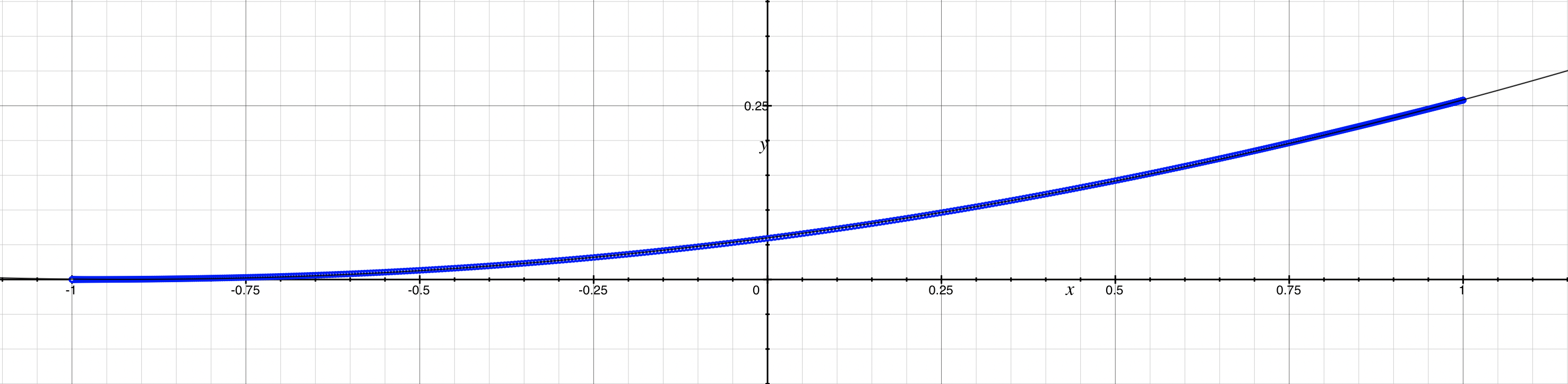 |
| The polynomial fit (black) against the true value of the function (blue) |
With that fit, we can evaluate both radiance and irradiance from an Ambient Dice SRBF basis in any direction.
The remaining problem is to evaluate specular from those same lobes. I don’t claim to have an ideal solution here (nor, for that matter, do I claim that the Ambient Dice basis function is a great choice for representing specular, since it’s inherently fairly low-frequency); however, I do have a general approach that could be useful.
Firstly, note that evaluating specular for a mirror-like surface is the same as evaluating the radiance in the mirror reflection direction. This observation allows us to approximate mirror specular indirect and diffuse lighting.
Let’s say we want to use the basis to evaluate specular for a range of roughness values. Well, it turns out that rough specular is fairly accurately approximated by multiplying the diffuse lighting by the specular BRDF response (which should be 1 if it’s energy conservative). For values in the middle of the roughness range, I found that blending between the two extremes – mirror reflectance and BRDF-multiplied diffuse – with the help of a 2D lookup table (roughness vs. viewing angle) actually works fairly well.
I won’t go into the details of my specular fit here – that will come in a future post, or you can look at Chapter 8 of my thesis (page 124). The part I want to emphasise is that, since all the RBF lobes share the same basis function, we only need one lookup table! We couldn’t do this for e.g. spherical harmonics since each SH band is evaluated differently – this is in fact a problem Chen and Liu ran into when using spherical harmonics for specular in the Lighting and Material of Halo 3.
The diffuse and specular fits in combination make a good-quality, efficiently-reconstructed method of storing low-frequency indirect diffuse and specular lighting. Although I haven’t tried, I’m sure you could get even better results with a 3D lookup table or different radial basis functions – for example, \((s \cdot v_i)^6\) or higher powers of cosine are an obvious choice to preserve higher-frequency information.
In the next post, I go into more detail about my fit for Ambient Dice specular.
-
The dot product is the element-wise sum of two vectors \(a\) and \(b\), and is equal to the length of \(a\) times the length of \(b\) times the cosine of the angle between them. ↩
-
Storing radiance rather than irradiance means more coefficients are required for runtime reconstruction; rather than only retrieving the coefficients for the non-zero basis functions in the sample direction, we need to retrieve coefficients for any lobe which may have influence over the hemisphere around the sample direction (which, in practice, usually means we need to use all of the lobes). ↩