Before we get into the technique: why might you want to use this? Perhaps you want specular lightmaps, have been considering spherical Gaussians, but want something cheaper and generally higher quality; this provides that.

Alternatively, you might currently store radiance for light probes in order-2 spherical harmonics (with 9 coefficients per colour channel) and would like indirect specular from them; for three more coefficients per channel, you can store radiance in the Ambient Dice format and get both diffuse and specular lighting with this technique.

For rough materials, this technique could even replace specular cubemaps; you could choose or blend between the Ambient Dice specular, light probes, and screen-space reflections based on roughness.

In the last post, I introduced the idea of using the Ambient Dice basis function for both diffuse and specular irradiance, and briefly described my method for the fit. This post will cover the specular fit in more detail. While it focuses on the Ambient Dice SRBF basis function and single-scattering GGX specular, it should be fairly straightforward to extend to other basis functions (particularly cosine-lobe-based ones) or BRDFs.

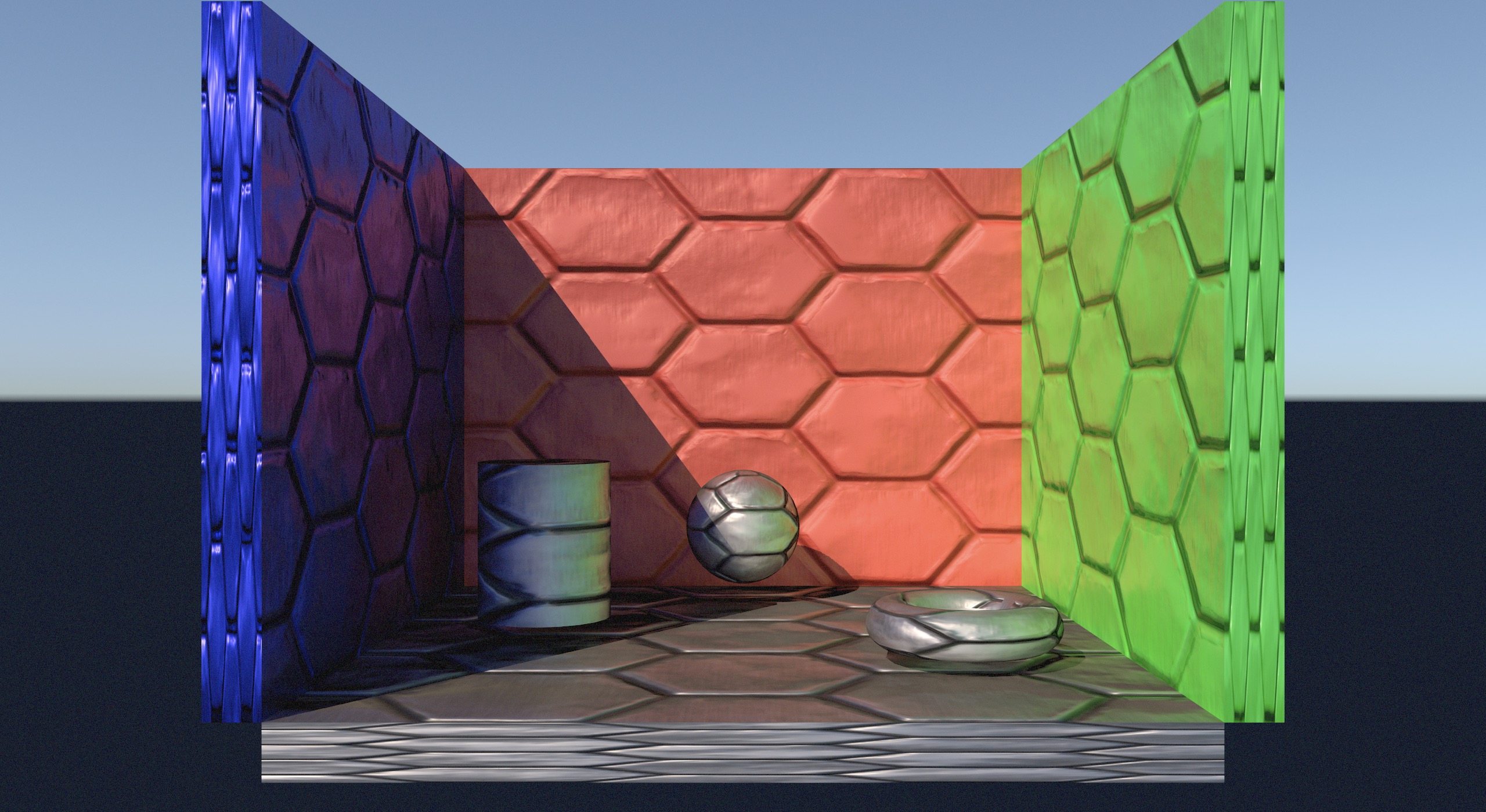
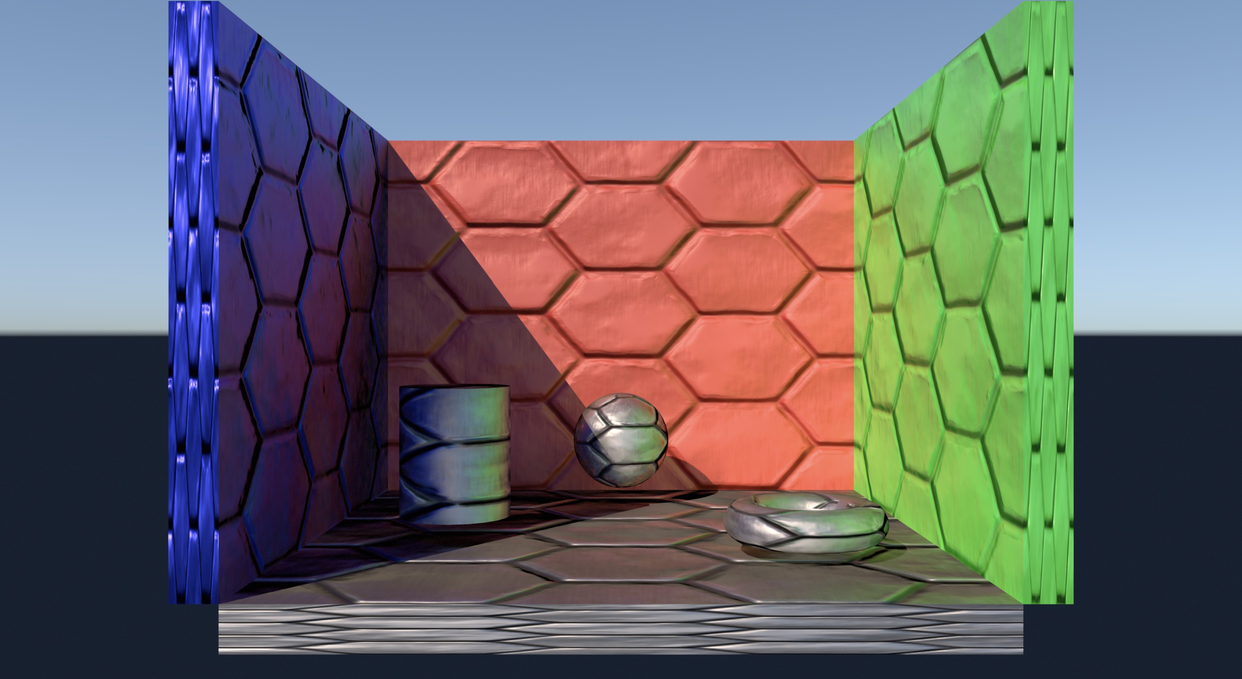
The ShaderToy below shows my fit against the reference (note: I’ve tested this to work in Firefox and Chrome, but it doesn’t appear to display in Safari):

ShaderToy link with source code

The left half of the sphere is the approximation, and the right half is the ground truth, where green is the f0 and blue is the f90 material scale factor. The sphere is parameterised by viewing direction; the edges of the sphere are at grazing angles, while the centre is viewing along the normal. The red dot is the lobe direction; you can move it around the sphere by dragging up and down with the mouse. Dragging left to right will change the surface roughness.

In general, finding the integral of a specular BRDF with illumination from an arbitrary basis function is a difficult problem due to the large number of free parameters. For a general specular model parameterised by some isotropic roughness \(\alpha\), normal direction \(n\), and reflectance at normal and grazing angles \(f_0\) and \(f_{90}\), the illumination from a light source in some linear basis is given by:

\[C_j(\omega_o ) = \int_\Omega B_i(\omega_i ) f_{br}(\alpha, \omega_i, \omega_o, n, f_0, f_{90}) d\omega_i\]

As far as I’m aware, there’s no closed-form solution to this integral for the GGX BRDF that I use for specular¹. Instead, we can either use Monte-Carlo integration to evaluate it, or we can use a fitted approximation or lookup table. Unfortunately, using Monte Carlo integration for this is overly expensive for real-time applications; visual artefacts are still readily apparent with as many as 32 samples when estimating \(C_j(\omega_o )\) – try setting sampleCount to 32 in groundTruth in the ShaderToy to see this in effect.

However, it is possible to derive a reasonably good fit to the specular irradiance. There are three key observations that we can use:

For a perfectly smooth specular reflector with the roughness parameter \(\alpha\) approaching zero, the BRDF becomes a delta function oriented in the surface’s reflection direction (given the view direction). The radiance in this case is just the basis function evaluated in the reflection direction multiplied by the Fresnel response.
For a very rough surface, the specular response will approach a Lambertian diffuse response. It so happens that in this case, scaling the diffuse irradiance by the BRDF’s response in a split-sum approximation (as inspired by Karis’ Real Shading in Unreal Engine 4) is a reasonably close match to the ground truth:
\[C_j(\omega_o ) \approx (\int_\Omega B_i(\omega_i ) d\omega_i) (\int_\Omega f_{br}(\alpha, \omega_i, \omega_o, n, f_0, f_{90}) d\omega_i)\]
We can use a lookup texture to store the BRDF response for different viewing directions and across the roughness range in a manner similar to Karis’ approach for image-based lighting.

Theres observations enable us to evaluate the specular irradiance at the two extremes of the roughness spectrum. The most obvious thing to do for the middle, therefore, is just to blend between them.

Unfortunately, using the split-sum approximation across the entire range gives fairly poor results – separating out the BRDF from the basis function response only really works for high roughnesses. Let’s take a step back and assume that we don’t have a lookup table at all. In that case, the best we can do is perform a parameterised lerp between the fully smooth response and the fully rough diffuse response, which could look something like this:²

float2 ApproximateAmbientDiceLobeSpecular(float3 lobeDirection, float3 viewDirection, float ggxAlpha) {
    float NdotLobe = dot(normal, lobeDirection);
    
    float3 reflectionDir = reflect(-viewDirection, normal);
    float RdotLobe = dot(reflectionDir, lobeDirection);
    
    float basisInMirrorDir = AmbientDiceCosineBasisFunction(RdotLobe);
    
    float diffuseParam = lerp(RdotLobe, NdotLobe, saturate(ggxAlpha));

    float diffuse = EvaluateAmbientDiceLobeDiffuse(diffuseParam);

    return lerp(basisInMirrorDir, diffuse, saturate(ggxAlpha));
}

This is obviously going to be fairly inaccurate – we’re not accounting for the specific BRDF response at all. To fix this, we can reintroduce the lookup table; however, rather than storing the BRDF response, the table instead stores whatever value will make our approximation match the true value – in other words, the lookup table stores the true value divided by the lerped approximation. This means that we can just multiply our approximation by the lookup table’s value to get the true irradiance value.

Let’s bring that into the code snippet above. Note that this time I’ve included my fitted parameters for the interpolation;³ I chose a quartic in \(\sqrt{\alpha}\), but it’s quite likely that there are better possibilities.

const float parameters[8] = { 3.0498910522220495, -6.983002509990005, 7.388270435580356, -2.662756921813306, -0.4005429486854629, 5.626699351644211, -6.040098716506305, 1.9006124935607012 };

float EvaluateAmbientDiceLobeDiffuse(float cosTheta) {
    return 0.05981 + 0.12918 * cosTheta + 0.07056 * cosTheta * cosTheta;
}

float EvaluateAmbientDiceLobeSpecular(float3 lobeDirection, float3 viewDirection, 
                                      float ggxAlpha) {
    float NdotLobe = dot(normal, lobeDirection);
    
    float3 reflectionDir = reflect(-viewDirection, normal);
    float RdotLobe = dot(reflectionDir, lobeDirection);
    
    float basisInMirrorDir = AmbientDiceCosineBasisFunction(RdotLobe);
    
    float sqrtAlpha = sqrt(ggxAlpha);

    float focusLerp = parameters[0] * sqrtAlpha + parameters[1] * ggxAlpha + 
                      parameters[2] * sqrtAlpha * ggxAlpha + parameters[3] * ggxAlpha * ggxAlpha;
    float diffuseParam = lerp(RdotLobe, NdotLobe, saturate(focusLerp));

    float diffuse = EvaluateAmbientDiceLobeDiffuse(diffuseParam);
    
    float alphaLerp = parameters[4] * sqrtAlpha + parameters[5] * ggxAlpha + 
                      parameters[6] * sqrtAlpha * ggxAlpha + parameters[7] * ggxAlpha * ggxAlpha;
    return lerp(basisInMirrorDir, diffuse, saturate(alphaLerp));
}

void evaluate() {
    float2 lutValue = AmbientDiceLUTValue(NdotV, ggxAlpha);

    float3 specularIrradiance = float3(0.0);
    for lobe in lobes {
        specularIrradiance += EvaluateAmbientDiceLobeSpecular(lobe.direction, V, 
                                                              ggxAlpha, lutValue)
    }
    specularIrradiance *= materialF0 * lutValue.x + materialF90 * lutValue.y;
}

That’s all great – we now have a simple and efficient way of evaluating the specular irradiance from an Ambient Dice lobe at runtime. However, if you’ve been following closely, you’ll notice that we’ve still got a problem. The lookup table still needs to somehow capture all of the free parameters of the integral – the angle between the normal and viewing direction, the BRDF roughness parameter, and the two angles between the viewing direction and the lobe (since both \(\theta\) and \(\phi\) affect the result).

To work around this, we can approximate by using a fixed lobe direction for each roughness value, using the assumption that the scale contained in the lookup table is reasonably independent of the lobe rotation. Doing so allows us to reduce the lookup table to be two-dimensional, parameterised by the roughness \(\alpha\) and the cosine of angle between the normal and viewing direction NdotV in the same manner as Karis’ split-sum for IBLs. While this assumption doesn’t generally hold, it gives fairly good results in practice.⁴

This approach also means that the lookup table value is independent from the lobe direction, requiring only a single texture lookup per pixel (rather than one per pixel per lobe). The lerp parameters in EvaluateAmbientDiceLobeSpecular are also independent of the lobe direction and so can be factored out, making the per-lobe evaluation very inexpensive.

For the choice of lobe direction, I use an approximation from Moving Frostbite to Physically Based Rendering for the dominant reflection direction for GGX – for smooth surfaces, this is the mirror reflection direction, while for rough surfaces this becomes aligned with the normal. The idea was to capture the response most accurately where the basis function would have highest intensity; however, it could be interesting to try different choices for the lobe direction to see how it affects the overall fit.

float3 GGXDominantDirection(float3 N, float3 R, float roughness) {
    float smoothness = saturate(1.f - roughness);
    float lerpFactor = smoothness * (sqrt(smoothness) + roughness);
    return normalize(lerp(N, R, lerpFactor));
}

float2 IntegrateLUTAmbientDice(float NdotV, float ggxAlpha) {
    const uint sampleCount = 256u;
    const float sampleScale = 1.f / float(sampleCount);
    
    const float3 normal = float3(0, 0, 1);
    
    float3 viewDirection = float3(0, sqrt(1.f - NdotV * NdotV), NdotV);
    float3 R = reflect(-viewDirection, normal);
    float3 lobeDirection = GGXDominantDirection(normal, R, ggxAlpha);
    
    float fittedValue = EvaluateAmbientDiceLobeSpecular(lobeDirection, 
                                                        viewDirection, 
                                                        ggxAlpha);
    
    float2 groundTruth = float2(0.0); // for f0 and f90MinusF0
    for (uint sampleIt = 0u; sampleIt < sampleCount; sampleIt += 1u) {
        float2 sampleUV = hammersley2D(sampleIt, sampleCount);
        float3 H = sampleGGXVNDF(viewDirection, ggxAlpha, ggxAlpha,
                                 sampleUV.x, sampleUV.y);
        float3 lightDirectionTangent = reflect(-viewDirection, H);
        
        float Vis = SmithGGXMaskingShadowingG2OverG1Reflection(viewDirection, 
                                                              lightDirectionTangent, 
                                                              H, ggxAlpha);
        
        float f0Weight = 1.f;
        float f90MinusF0Weight = pow(1.f - saturate(dot(viewDirection, H)), 5.f);
        
        float basis = AmbientDiceCosineBasisFunction(
                        dot(lobeDirection, lightDirectionTangent)
                      );
        
        float2 brdf = float2(f0Weight - f90MinusF0Weight, f90MinusF0Weight) * 
                        Vis;
        if (lightDirectionTangent.z > 0.f) {
            groundTruth += basis * brdf * sampleScale;
        }
    }
    
    return groundTruth / fittedValue;
}

The lookup table generation uses Heitz’s method for Sampling the GGX Distribution of Visible Normals; look there or at the source code for the ShaderToy attached to this post for the full source code.

Diffuse Fits for Cosine-Lobe Basis Functions

The specular solution depends on having a diffuse fit for the basis function. I’ve found polynomial fits for the Ambient Dice cosine-lobe basis function, where \(s\) is the normal direction and \(v_i\) is the lobe direction:

\[\cos(\theta) = (s \cdot v_i) \\ B_i(s) = 0.35 \max(\cos(\theta), 0)^2 + 0.25 \max(\cos(\theta), 0)^4\]

along with for basis functions created from increasing powers of clamped cosine. The quadratic fits are of the form \(f(x) = a + bx + cx^2\), where \(x = \cos(\theta)\), while the quartic fits are of the form \(f(x) = a + bx + cx^2 + ex^4\). Note that the \(x^3\) term had negligible contribution in all of the fits and was therefore dropped.

Note that the basis functions use the clamped cosine term (i.e. \(\max(s \cdot v_i, 0)^n\)) , while the fits use the unclamped cosine (i.e. \(s \cdot v_i\)).

The fits are:

Ambient Dice (0.35x^2 + 0.25x^4) (Quadratic Fit) (RMSE = 0.00039830040057973803, max delta = 0.0011889899178523927):
(a: 0.059806690913006784, b: 0.12917904381845316, c: 0.07056134282329878)

Ambient Dice (0.35x^2 + 0.25x^4) (Quartic Fit) (RMSE = 2.2924203751463493e-06, max delta = 5.9859991145602e-06):
(a: 0.05935860814656071, b: 0.12917904381815673, c: 0.07503324753667442, e: -0.005206825865963849)

x^2 (Quadratic Fit) (RMSE = 3.0408681122397585e-06, max delta = 6.544694088506109e-06):
(a: 0.12496957942811276, b: 0.25002412959296777, c: 0.1250610948589435)

x^2 (Quartic Fit) (RMSE = 3.0405945870056214e-06, max delta = 6.423524563908889e-06):
(a: 0.1249695335534175, b: 0.2500241295938416, c: 0.12506155284179532, e: -5.33276807285143e-07)

x^4 (Quadratic Fit) (RMSE = 0.001593126030041, max delta = 0.004746797107934839):
(a: 0.06426935244942271, b: 0.1666823938414644, c: 0.10715983849997654)

x^4 (Quartic Fit) (RMSE = 5.021965714382778e-06, max delta = 1.4951021221017158e-05):
(a: 0.062477085624468985, b: 0.16668239384246453, c: 0.12504681624769828, e: -0.02082655700848173)

x^6 (Quadratic Fit) (RMSE = 0.0021760428533152162, max delta = 0.005930189360399074):
(a: 0.041656708863260575, b: 0.12501163876845992, c: 0.08928511926559841)

x^6 (Quartic Fit) (RMSE = 0.0001519926731062455, max delta = 0.0005550233310728514):
(a: 0.039214627502226256, b: 0.12501163876761548, c: 0.11365730224790668, e: -0.02837755296728098)

x^8 (Quadratic Fit) (RMSE = 0.0023537857692170917, max delta = 0.0060368080144615754):
(a: 0.030296404520220775, b: 0.10000916682096359, c: 0.07574957031520438)

x^8 (Quartic Fit) (RMSE = 0.0002839638757536194, max delta = 0.0009460013572480663):
(a: 0.027667723047883053, b: 0.10000916682187795, c: 0.10198403855930246, e: -0.03054588966300734)

If you’re interested in sharp specular highlights (as you might get from spherical Gaussians with high \(\lambda\) values) then using a basis function like \(B_i(s) = \max(\cos(\theta), 0)^8\) might be a good fit; note, however, that this means your environment map may start to look like a series of point lights, as it does with spherical Gaussians, and the accuracy of diffuse irradiance will likely suffer.

Results

The table below compares spherical Gaussians (\(\lambda = 6\)) with 9 or 12 lobes against Ambient Dice with 9 or 12 lobes (where the nine-lobe variant contains only the lobes oriented towards the upper hemisphere) on the Ennis environment map. The spherical Gaussians use an anisotropic spherical Gaussian fit for specular as detailed by MJP.

	Reference	AD9	AD12	SG9	SG12
Radiance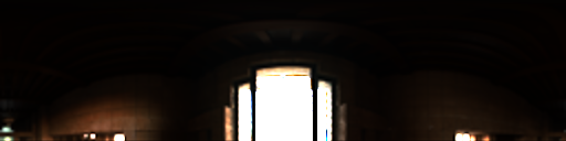
RMSE	-	5.25	5.83	6.45	5.54
Lambert
RMSE	-	0.148	0.105	0.327	0.225
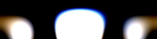
GGX \(\alpha = 0.1\)
RMSE	-	2.17	2.74	2.97	2.34
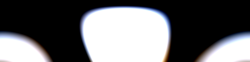
GGX \(\alpha = 0.2\)
RMSE	-	0.947	1.37	1.47	1.12
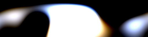
GGX \(\alpha = 0.4\)
RMSE	-	0.276	0.409	0.566	0.574
GGX \(\alpha = 0.6\)
RMSE	-	0.130	0.137	0.378	0.466
GGX \(\alpha = 0.8\)
RMSE	-	0.119	0.091	0.299	0.374

More comparisons of this type on a wide range of environment maps are available in Appendix C of my thesis.

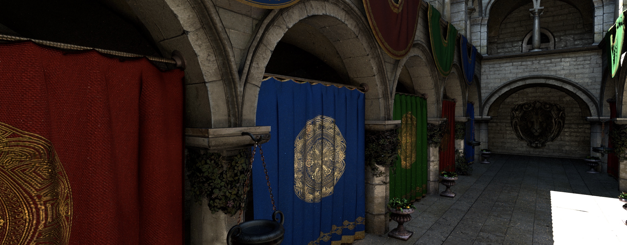
Indirect lighting from baked lightmaps in Crytek Sponza with only single-scattering GGX specular materials

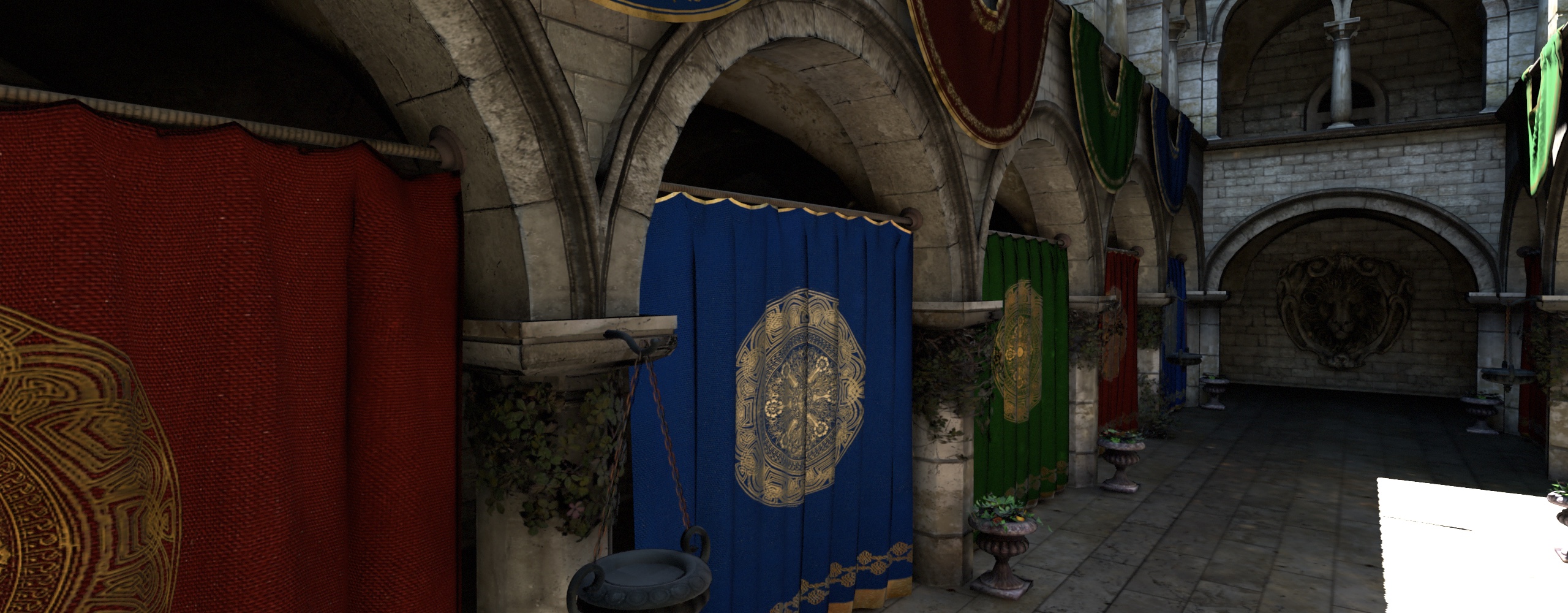Non-negative hemispherical Ambient Dice (nine lobes) (0.9ms per frame)

Path-traced reference

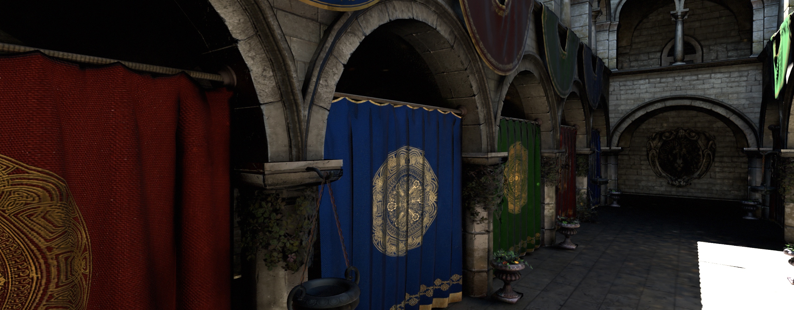Non-negative spherical Gaussians (twelve lobes, \(\lambda = 8\)) (2.5ms per frame)

The Baking Lab scene using indirect illumination lightmaps

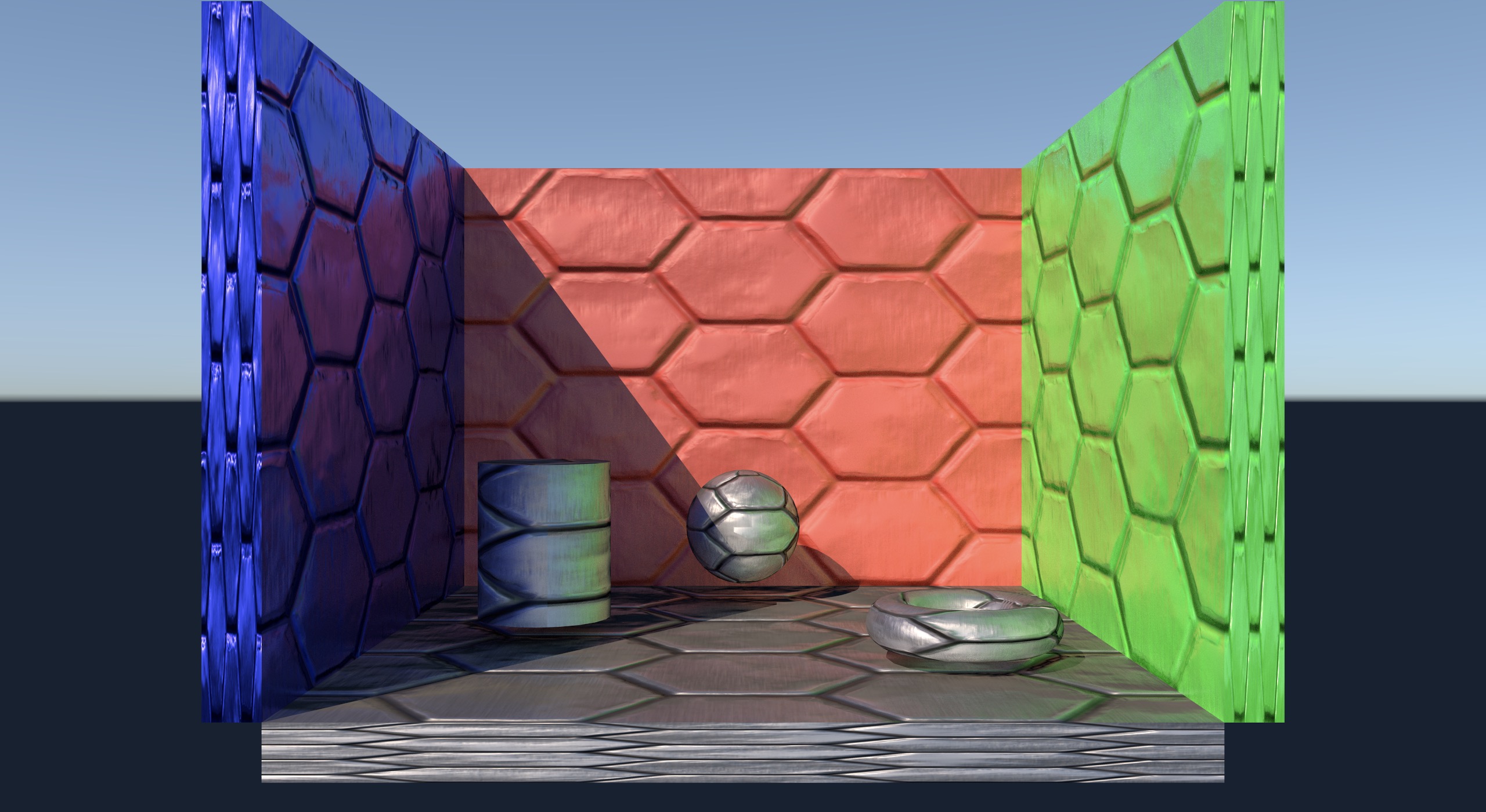Path-Traced Reference

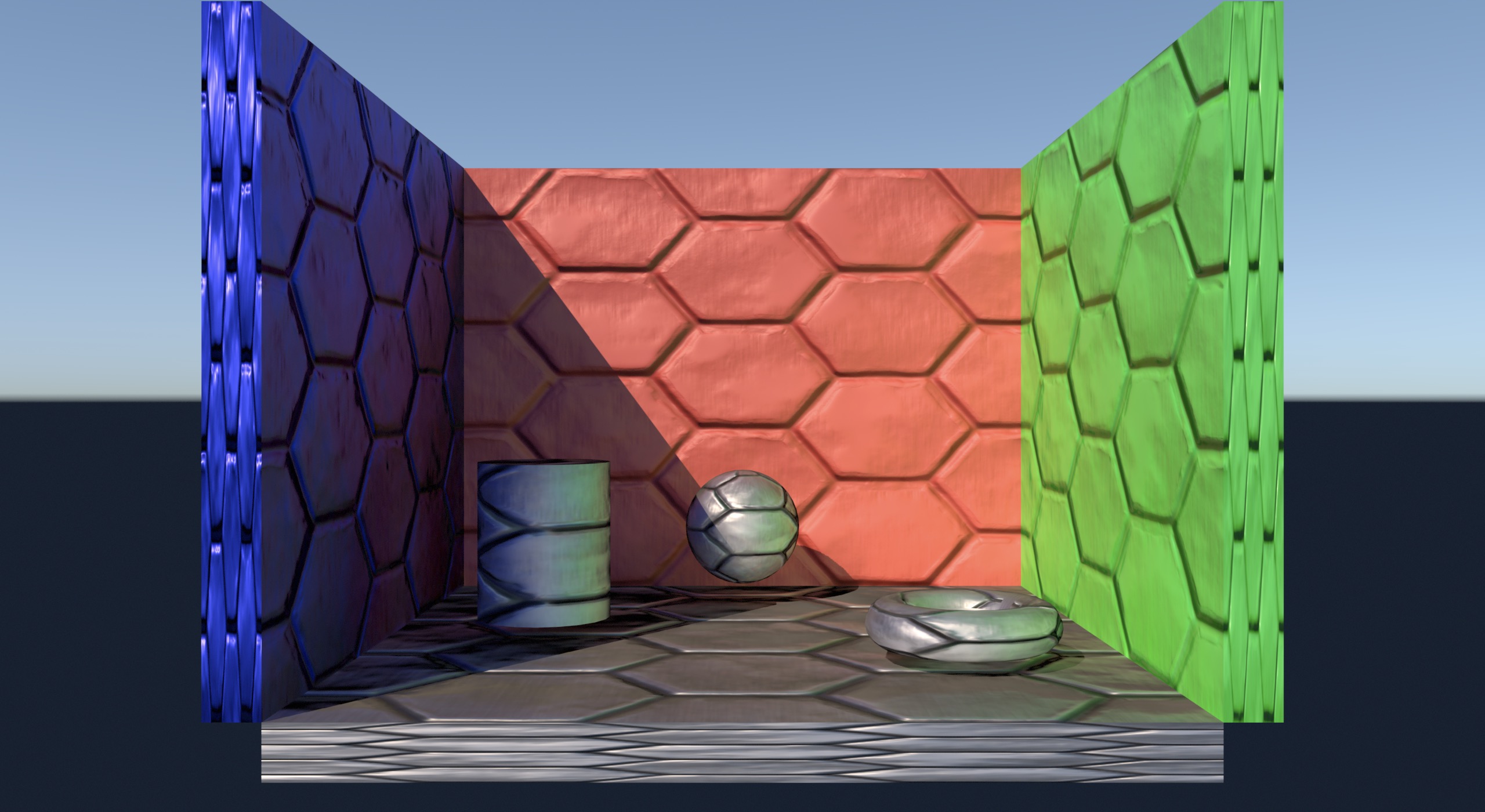Hemispherical Ambient Dice (nine lobes)

Hemispherical Ambient Dice (nine lobes) with screen-space reflections

Spherical Gaussians (twelve lobes)

Spherical Gaussians (twelve lobes) with screen-space reflections

More precisely, this fit is for the single-scattering GGX specular model using the Smith height-correlated masking-shadowing function; Heitz provides details in Understanding the Masking-Shadowing Function in Microfacet-Based BRDFs. ↩
We can do better than directly using ggxAlpha for the lerp parameter; this code snippet is just for the sake of example. ↩
I used MPFIT to find the parameters that minimised the error of my LUT-multiplied approximation over the parameter space. ↩
One possibility would be to use a 3D lookup table, with the angle between the normal and lobe direction as the third coordinate for the table. I was happy enough with the quality of the 2D LUT that I didn’t feel the need to try this. ↩